Geographic Information - Rasterize Twitter Data Tutorial
A common task in machine learning is to transfer point objects like Tweets or points in OpenStreetMap into a form that is suitable for machine learning together with satellite or aerial imagery or other raster graphics. There are many good ways of doing so, but this article will concentrate on one of the easiest ways of doing it through the excellent R packages sp and raster.
The overall structure of this example is that we first load a GeoTiff raster file for our raster reference. This can be any georeferenced raster and will be used mainly as a template for the metadata of the raster (e.g., projection, coordinates, extent, etc.). This raster is then filled with new values, filtered with various basic approaches and can be written to another GeoTiff file or consumed directly, for example, as a matrix.
Preparations
In order to setup your system, you need to have a recent installation of R (possibly RStudio, if you like). From the prompt, you can install the two packages raster and sp, if you don’t have them yet.
install.packages("raster")
install.packages("sp");
When these are installed, you can load them via
library(raster)
Loading the template
Loading the template file is now a single line:
r = raster("grid_100m.tif")
Note that R is not loading the raster data with this call. Instead, the raster data will only be loaded if it is consumed. But, the object r now contains all the needed information about the raster.
> print(r)
class       : RasterLayer
dimensions  : 988, 1160, 1146080  (nrow, ncol, ncell)
resolution  : 100, 100  (x, y)
extent      : 390280, 506280, 5361520, 5460320  (xmin, xmax, ymin, ymax)
coord. ref. : +proj=utm +zone=31 +datum=WGS84 +units=m +no_defs +ellps=WGS84 +towgs84=0,0,0
data source : /data/datasets/dase-lcz/train/paris/grid/grid_100m.tif
names       : grid_100m
values      : 1, 1146080  (min, max)
You can see the dimensions, the resolution, extent, and coordinate reference system, the data source, the name, and the value range. Note that a raster in R has a single layer only. However, if the file was containing more than one layer, the raster library would return a RasterBrick object, which represents a stack of rasters.
Extracting the Extent in WGS84 for Finding the Right Tweets
We now want to get the WGS84 bounding box of the raster. This is pretty easy in R:
e = as(extent(r),"SpatialPolygons")
proj4string(e) = proj4string(r)
wgs="+proj=longlat +datum=WGS84 +no_defs +ellps=WGS84 +towgs84=0,0,0"
e = extent(spTransform(e,CRS(wgs)))
One gets the extent of a raster from the extent function. However, this is not a spatial object, but can be casted into a polygon, which leads to the first line. As the extent was not a spatial object, it does not carry projection information and neither does the polygon we just cretaed. Therefore, we add projection information with the second line. The third line defines the projection we are interested in (it is WGS84, because we want to filter Tweet objects, which can have spatial information in this projection. The last line now composes a coordinate transformation spTransform and extracts the extent of the Polygon. This means that we now have a valid bounding box even though the polygon will not be axis parallel after coordinate transformation.
Let us have a short look:
> print(extent(r))
class       : Extent
xmin        : 390280
xmax        : 506280
ymin        : 5361520
ymax        : 5460320
> print(e)
class       : Extent
xmin        : 1.491239
xmax        : 3.086372
ymin        : 48.39729
ymax        : 49.29559
And let us find the center to create a link to Google Maps for looking at where this raster is actually located. Casting an extent to a matrix gives it as a two by two matrix:
> print(as.matrix(e))
    min       max
x  1.491239  3.086372
y 48.397287 49.295594
and a column-wise mean returns the center
> apply(as.matrix(e),1,mean)
        x         y
 2.288805 48.846441
This seems to be Paris: https://www.google.com/maps/place/48.846441,2.288805
Extracting Tweets
Tweets (just as many modern Internet APIs) are given in form of Javascript Object Notation (JSON). If you are managing datasets of tweets, the easiest way is to have tweets in a file, each tweet given as a JSON object consuming a line. Then, the JSON Query Engine JQ is flexible enough and powerful to manipulate and organize this data, we will give some examples.
First, of course, we need to find objects that fall into the region of the raster. This is as easy as writing a JQ query in which we first select all JSON objects for which .coordinates is not null (see the API docs) and from those, we select those that have suitable coordinates in relation to the WGS84 extent of our raster.
> filter = sprintf("jq -c \"select(.coordinates != null) |select (.coordinates.coordinates[0] >= %f and .coordinates.coordinates[0] <= %f and .coordinates.coordinates[1] >= %f and .coordinates.coordinates[1] <= %f )\"",e[1],e[2],e[3],e[4])
> print(filter, quote=F)
 [1] jq -c "select(.coordinates != null) |select (.coordinates.coordinates[0] >= 1.491239 and .coordinates.coordinates[0] <= 3.086372 and .coordinates.coordinates[1] >= 48.397287 and .coordinates.coordinates[1] <= 49.295594 )"
This is now a shell command, which can be used to actually transform a dataset and this is, how this can be done given a BZIP2-compressed file with one JSON object on each line.
bzcat tweets.json.bz2 | jq -c "select(.coordinates != null) |select (.coordinates.coordinates[0] >= 1.491239 and .coordinates.coordinates[0] <= 3.086372 and .coordinates.coordinates[1] >= 48.397287 and .coordinates.coordinates[1] <= 49.295594 ) |bzip2 > paris.json.bz2
This now decompresses the tweets.json.bz2 collection, selects all tweets that are georeferenced and inside the raster, compresses the output and writes a file paris.json.bz2 containing exactly the interesting tweets from the dataset.
Transforming JSON to SSV
Now, though R can read JSON, we can make our live easier by using JQ a second time to extact some features and write a space-separated value file usable with read.table function.
transformer="jq -cr '(.coordinates.coordinates[0]|tostring)+\" \"+(.coordinates.coordinates[1]|tostring)+\" \"+(.user.friends_count |tostring)' "
print(transformer, quote=F)
[1] "jq -cr '(.coordinates.coordinates[0]|tostring)+\" \"+(.coordinates.coordinates[1]|tostring)+\" \"+(.user.friends_count |tostring)' "
system(sprintf("bzcat paris.json.bz2 | %s > feature.dat" , transformer))
This is now inside R, we first create a transformer that selects the coordinates (as a string) and joins them through the + operator. This generates a line with longitude, latitude, and friends_count. Note the -r flag to JQ: JQ is usually outputting JSON and the representation of a string in JSON is escaped. But as we want plain strings, we can tell JQ that it should not escape single strings but give them as they are. Otherwise, you see coloured strings.
Bring this into the Raster
We now nead to load the feature file with the coordinates, tell R that it is a spatial object and give the projection:
A = read.table("feature.dat")
colnames(A) = c("lon","lat","friends_count")
coordinates(A) = ~lon+lat;
proj4string(A) = wgs
Now, A is a spatial object, but it is in the wrong projection. If we would now try to use it together with the raster, we would see errors accordingly. Now, again, spTransform is our friend:
A = spTransform(A, proj4string(r))
Now, A is a SpatialPointsDataFrame (that is a data.frame with spatial information) and it is in the same projection as the raster. We can now populate the raster from this object through the rasterize function. Let us take the mean friends_count in each cell:
s = rasterize(A, r, "friends_count",mean)
This now assigns to each cell of r the mean of the vector of all friends_count column of the data.frame A. Cells that don’t receive any points are assigned with a value of NA, we take care of removing this later. You can now plot this raster through
plot(s)
Note that you can write your own function for rasterize() that transforms the subset of the data.frame into a single value given to the cell.
A little bit of processing on the raster
There are many ways of doing sensible operations to the raster and, again, the raster package makes this extremely intuitive with R. The following examples just show very basic operations that you can take as a starting point for your own raster processing.
A Sum Filter
This filter takes the sum of all neighbors according to the matrix. That is a grid of 5x5 neighboring pixels is summed up.
filter.size=5
s2 <- focal(s, w=matrix(1,nrow=filter.size,ncol=filter.size)  , fun=sum, na.rm=T)
plot(s2)
A Gaussian Filter
Writing standard filter matrices by hand is annoying, therefore, focalWeight generates a few:
s2 <- focal(s, w=focalWeight(s,filter.size,'Gauss')  , fun=sum, na.rm=T)
plot(s2)
Aggregation
The resolution might be too high, just applying an aggregate function (mean below) to rectangles returning a single value in a lower resolution raster is standard:
s2 <- aggregate(s, fact=5, fun=mean, expand=TRUE)
plot(s2)
Doing your own
The following illustrates, how you can do your own transformations. This transformation now fills NAs with the mean of the 3x3 neighbors. If this is also NA because the neighbors did not provide suitable information for a mean, we set it to zero.
fill.na <- function(x, i=5) {
    if( is.na(x)[i] ) {
        val = mean(x, na.rm=TRUE);
        if (is.na(val))
        {
            val = 0;
         }
    return( val )
  } else {
      return (x[i])
  }
}
Applying this function is as easy as:
s2 <- focal(s, w = matrix(1,3,3), fun = fill.na,
        pad = TRUE, na.rm = FALSE )
Finally, let’s have an image of this feature in Paris with only a few tweets:
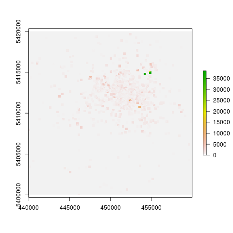
We hope this micro-tutorial is helpful for you.
Downloads
| Author: | Artem Leichter |
| Last modified: | 2018-10-08 |