> Data science course by AMA & ICAML - Practical Part

Machine Learning

In this chapter we will train a classification and regression model on the cleaned dataset. To that end, we use the sklearn module from scipy (scientific Python) framework.

Predicting the survivors (Classification)

First, we train a classification model. In particular we compare a decision tree to a random forest and a support vector machine. Further information on the principle concepts of these methods can be found on the icaml pages for Decision Trees, Random Forests and Support Vector Machine.

Let’s recall the available attributes:

import pandas as pd

table = pd.read_csv('titanic_cleaned.csv', sep=';')
print(list(table.columns))

['Survived', 'Pclass', 'Sex', 'Age', 'SibSp', 'Parch', 'Fare', 'Embarked']

Here we choose the attribute survived as target variable Y, which should be predicted. All other attributes are used as indicators (input of the model X)

import numpy as np

Y = table.values[:,0].astype(np.bool) # variable that should be predicted
X = table.values[:,1:-2]                # model inputs (indicators)

Decision Tree

The concept of a Decision Tree is actually very simple:Basically we have a tree-like structure (nodes connected with edges) starting with a root node. Each node (including the root) has two successor nodes except for the so called leaves which do not have any successor. Starting from the root node, any sample (indicator vector) is evaluated at each node based on a fixed decision. Depending on the outcome of this decision, the sample is forwarded to one of the successors until it reaches a leaf node. The leave then indicates the class.

Training of such a tree is based on training examples which are used to find the best decisions and determine the leaves classes. Simply spoken this is based on try and error until a good configuration is found.

We use the implementation from the skklearn module:

from sklearn import tree

The model can be created and trained with only two lines of code. We use entropy for the optimization of the decisions and set the number of leaf nodes to 12 (for visualization purpose). The function fit() traines the model on the given samples and scores computes the accuracy on our data.

from matplotlib import rcParams, pyplot as plt

rcParams['figure.figsize'] = [6,4]
dtc = tree.DecisionTreeClassifier(criterion='entropy', max_leaf_nodes=12)
dtc.fit(X, Y)

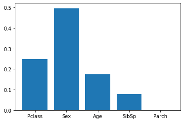
plt.bar(list(table.columns)[1:-2],dtc.feature_importances_ )
plt.show()

print("Classification accuracy is {:.1%}".format(dtc.score(X,Y)))

Classification accuracy is 82.6%

Decision trees have the nice property, that they can be visualized nicely. This is demonstrate in the next cell.

rcParams['figure.figsize'] = [14,13] # with and height of plots (default is 6,4 )
t = tree.plot_tree(dtc,feature_names=list(table.columns)[1:],
                   class_names=['Dead', 'Survived'], filled=True, 
                   proportion=True, impurity=False, precision=1)

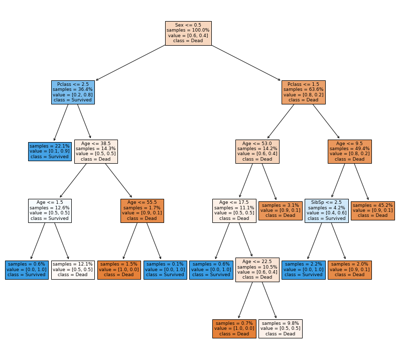
We can guess that the most important feature is the sex, since this is used in the root node. To make sure, we can check for the feature importances.

importances = dtc.feature_importances_
print(list(table.columns)[1:])
print(importances)

['Pclass', 'Sex', 'Age', 'SibSp', 'Parch', 'Fare', 'Embarked']
[0.24892461 0.49646195 0.17509596 0.07951748 0.        ]

Can we do better?

The accuracy we got in the previous run was actually not very good. We limited the number of leaf nodes an thus the capacity of the model. Next, we run the tree without limitation (except the default values).

dtc = tree.DecisionTreeClassifier()
dtc.fit(X, Y)

print("Classification accuracy is {:.1%}".format(dtc.score(X, Y)))

Classification accuracy is 93.3%

Now our model fits the data almost without error, but..

What about overfitting?

If our goal is to create a generalizing model of rules about surviving the titanic, we have to make sure, that the model is not overfitting. The problem of overfitting can be imagined very simple. Imagine you are training a model to add two numbers, but you only train it one sample 1+2=3. The model will quickly learn that the correct output is 3 with 100 % accuracy. However, it will predict 3 regardless of the input, which means it actually just memorized the dataset.

Same thing can also occur with more complex scenarios. To counteract overfitting, one usually holds back a part of the data which is not used for training but only for validation of the model.

X_train, X_test = np.split(X, indices_or_sections=[500,])
Y_train, Y_test = np.split(Y, indices_or_sections=[500,])

dtc = tree.DecisionTreeClassifier()
dtc.fit(X_train, Y_train)

print("Classification accuracy on train set is {:.1%}".format(dtc.score(X_train, Y_train)))

Classification accuracy on train set is 93.8%

The training accuracy is still very good, but when we observe the score on the unseen test data, overfitting becomes obvious:

print("Classification accuracy on train set is {:.1%}".format(dtc.score(X_test, Y_test)))

Classification accuracy on train set is 79.7%

Random Forest

Keeping this problem in mind we switch to another classification model: the Random Forest, which is basically a combination of multiple Decision Trees. This combination makes the resulting model more complex, but also more robust!

from sklearn.ensemble import RandomForestClassifier
from sklearn.model_selection import GridSearchCV as GridSearch

Finding a good model using Grid Search with Cross Validation

In order to find good parameters w.r.t. the accuracy but also to the problem of overfitting, we use a strategy called Grid Search with Cross Validation. This means we are train models on multiple sets of parameters and evaluating each on data, which were not used for training. For each parameter set we rotate the training and validation data, so that the result is more robust.

# The fixed parameters are hold constant
fixed_parameters = {
    'max_features' : 'sqrt',   # Number of features considered per node: 'square rule'
    'criterion' : 'entropy'    # Splitting criterion: 'information gain'
}

# The tuned parameters are optimized during the grid search.
# Instead of a fixed value, we store a range of values for each variable
tunable_parameters = { 
    'n_estimators': [10,20,50],        # Maximum depth of the tree
    'max_depth': [10,20,50],        # Maximum depth of the tree
    'min_samples_split': [2,5,10]  # Min. number of samples in a node to continue splitting
}

# Create an instance of the model that will be optimized
model = RandomForestClassifier(**fixed_parameters)

# Create the optimizer and run the optimization
opt = GridSearch(model, tunable_parameters, cv = 3, scoring="accuracy", verbose=True)
opt.fit(X_train, Y_train)

# Save and print optimal parameters
opt_parameters = opt.best_params_
print("Best (tested) parameters:", opt_parameters)

Fitting 3 folds for each of 27 candidates, totalling 81 fits


[Parallel(n_jobs=1)]: Using backend SequentialBackend with 1 concurrent workers.


Best (tested) parameters: {'max_depth': 20, 'min_samples_split': 10, 'n_estimators': 10}


[Parallel(n_jobs=1)]: Done  81 out of  81 | elapsed:    2.4s finished

The best configuration (of the tested ones) is:

• Limit the depth of each tree to 50
• Don’t split a node if there are less than 10 samples in it
• Use 20 trees

rfc = opt.best_estimator_
print("Classification accuracy on train set is {:.1%}".format(rfc.score(X_train, Y_train)))

Classification accuracy on train set is 86.2%

print("Classification accuracy on train set is {:.1%}".format(rfc.score(X_test, Y_test)))

Classification accuracy on train set is 84.0%

Using this configuration, we reach a good classification accuracy also for the unseen data.

Predicting the Fare (Regression)

Besides classification models can be trained for regression. The difference is that instead of predicting a class, one or many values are predicted. We can use the dataset to predict the fare, using the other attributes as indicator variables.

Again using the sklearn module, we have access to several regression models. Here we use:

• Linear regression
• Regression Tree
• Regression forest

from sklearn.linear_model import LinearRegression
from sklearn.tree import DecisionTreeRegressor
from sklearn.ensemble import RandomForestRegressor
rcParams['figure.figsize'] = [6,3]

table = pd.read_csv('titanic_cleaned.csv', sep=';')
print(list(table.columns))

['Survived', 'Pclass', 'Sex', 'Age', 'SibSp', 'Parch', 'Fare', 'Embarked']

Yr = table.values[:,-2]    # Fare is target attribute
Xr =  table.values[:,1:4]  # Class, Sex and Age are indicator variables

Training a regression model works basically analogously to the classification model. We start with the linear regression model:

linreg = LinearRegression()
linreg.fit(Xr, Yr)
linreg.score(Xr, Yr)

0.3261251512029797

Second model is the Regression Tree:

dtr = DecisionTreeRegressor()
dtr.fit(Xr, Yr)

plt.bar(list(table.columns)[1:4], dtr.feature_importances_ )
plt.show()

dtr.score(Xr, Yr)

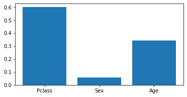
0.6017551780660924

Lastly, we train the Regression Forest:

rfr = RandomForestRegressor(n_estimators=200)
rfr.fit(Xr, Yr)

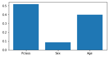
plt.bar(list(table.columns)[1:4], rfr.feature_importances_ )
plt.show()

rfr.score(Xr, Yr)

0.5910167154306933

Regarding the feature importances, all models yield similar results. We observe that the linear regression has a much lower score (here it’s the coefficient of determination). We can deduct, that the mapping from the used indicator variables to the fare is not linear.

Note, that we did not check for overfitting here!! This would work in the same way, than for classification.

In the next cell you can simulate some data and let the models predict the fare:

sample = [[1, 1, 29]] # Class Sex Age

fare = linreg.predict(sample)[0]
print(f'LinReg: The fare would have been {fare} dollar')

fare = dtr.predict(sample)[0]
print(f'RegTre: The fare would have been {fare} dollar')

fare = rfr.predict(sample)[0]
print(f'RegFor: The fare would have been {fare} dollar')

LinReg: The fare would have been 77.04723108265605 dollar
RegTre: The fare would have been 48.3 dollar
RegFor: The fare would have been 50.869049201587316 dollar

Following cell removes the input/output promts to the left of the cells. Output scroll toggle via ctrl-o.

%%HTML
<style>div.prompt {display:none}</style>