> Data science course by AMA & ICAML - Practical Part

Working with table data

Now that we introduced some very basic concepts of Python, we move on towards doing some data science. In the next part, we will tackle the following tasks:

• Reading and writing csv files
• Analyze and visualize specific attributes

Here we will use a dataset which contains information about the passengers of the titanic. Further information about the dataset here.

Read csv file

In the following cells we walk through an example for reading a csv file line by line and parsing the data into a list. As a reminder, a csv file is basically a text-file which contains values, separated by some delimiter which is usually a comma.

In the next cell the built-in function open() is used to read the file to the working memory. Here we use a so called context manager, that will automatically close the file afterwards. We use read_lines(), which gives us a list of all lines, each being a text, stored as string.

file_name = 'titanic2.csv'         # Specify file name (relative to this notebook)
with open(file_name, 'r') as file: # Load the document to file ('r' means 'reading mode')
    lines = file.readlines()       # Read all lines of the file
                                   # At this point the file is automatically closed
print('data type of lines:', type(lines))
print('data type of first element in lines:', type(lines[0]))

data type of lines: <class 'list'>
data type of first element in lines: <class 'str'>

Working with lists

Knowing that lines is a list we can e.g. check the number of elements, using len() or access specific entries by index. The indexing is done by passing the index as integer in square brackets. Note that the index starts from 0, as common in most programming languages.

num_lines = len(lines)             # Build in function 'len()' gives number of entries
print('number of lines:', num_lines)

first_line = lines[0]              # Using [] to index an element in list
print('\nLine 1:\n', first_line)
second_line = lines[1]              
print('Line 2:\n', second_line)  
third_line = lines[2]              
print('Line 3:\n', third_line)  

number of lines: 892

Line 1:
 PassengerId;Survived;Pclass;Name;Sex;Age;SibSp;Parch;Ticket;Fare;Cabin;Embarked

Line 2:
 1;0;3;Braund, Mr. Owen Harris;male;22;1;0;A/5 21171;7.25;;S

Line 3:
 2;1;1;Cumings, Mrs. John Bradley (Florence Briggs Thayer);female;38;1;0;PC 17599;71.2833;C85;C

As common for csv files, the first line is a so called header line, that describes the meaning and order of the stored attributes. E.g. the first value is the Passengers ID, the second value tells whether the passenger survived and so on.

When analyzing such a csv file it makes sense to take a look at the first few lines. E.g. the following questions are important:

• What attributes are stored? Do I know the meaning of all names?
• What delimiter is used to split the values?
• How are the values for each attribute stored? E.g. which data type is used?

Instead of explicitly accessing the first three lines, we can use a for-loop. This is shown in the next cell, where i loops from 0 to 7 (7 not included) and the corresponding line is printed.

for i in range(7):                 # Loop over indices: 0,1,2
    print(lines[i])

PassengerId;Survived;Pclass;Name;Sex;Age;SibSp;Parch;Ticket;Fare;Cabin;Embarked

1;0;3;Braund, Mr. Owen Harris;male;22;1;0;A/5 21171;7.25;;S

2;1;1;Cumings, Mrs. John Bradley (Florence Briggs Thayer);female;38;1;0;PC 17599;71.2833;C85;C

3;1;3;Heikkinen, Miss. Laina;female;26;0;0;STON/O2. 3101282;7.925;;S

4;1;1;Futrelle, Mrs. Jacques Heath (Lily May Peel);female;35;1;0;113803;53.1;C123;S

5;0;3;Allen, Mr. William Henry;male;35;0;0;373450;8.05;;S

6;0;3;Moran, Mr. James;male;;0;0;330877;8.4583;;Q

Exercise

Take a closer look to the previous output and try to answer the questions above. Can you detect any anomalies?

Working with strings

Now we have stored the data in the working space and know something about the structure, we continue by further splitting each line into it’s values. Since each line is stored as a string, we can use the built-in function split() which takes a delimiter and returns a list of all fragments. Again we can use indexing to access specific elements.

line_tokens = first_line.split(';') # Split the first line at each ';' > returns a list

print('Splitted list:\n', line_tokens)
print('\nFirst element:', line_tokens[0])

Splitted list:
 ['PassengerId', 'Survived', 'Pclass', 'Name', 'Sex', 'Age', 'SibSp', 'Parch', 'Ticket', 'Fare', 'Cabin', 'Embarked\n']

First element: PassengerId

Exercise

Loop over all elements in the list, split the line and print only the name of each passenger.

'''
for ... in ...:                     # loop over lines (start at second)
    line =
    entries = ...                   # split at ';'
    name = ...                      # get 'name' of entry
    print(...)                      # print name
'''
### BEGIN SOLUTION
for i in range(1, num_lines):      
    line = lines[i]
    entries = line.split(';')           
    print(entries[3])
### END SOLUTION

Braund, Mr. Owen Harris
Cumings, Mrs. John Bradley (Florence Briggs Thayer)
Heikkinen, Miss. Laina
Futrelle, Mrs. Jacques Heath (Lily May Peel)
Allen, Mr. William Henry
Moran, Mr. James
McCarthy, Mr. Timothy J
Palsson, Master. Gosta Leonard
Johnson, Mrs. Oscar W (Elisabeth Vilhelmina Berg)
Nasser, Mrs. Nicholas (Adele Achem)
Sandstrom, Miss. Marguerite Rut
Bonnell, Miss. Elizabeth
Saundercock, Mr. William Henry
Andersson, Mr. Anders Johan
Vestrom, Miss. Hulda Amanda Adolfina
Hewlett, Mrs. (Mary D Kingcome)     ...

Control structures

When writing complex programs, control structures are used to control code execution depending on conditions. To this end, we start by initializing two boolean variables. Recall, that booleans are logical variables that can have only two possible values - true or false.

A = True
B = False

print(type(A))

<class 'bool'>

Next the basic syntax of conditions is shown. It starts with the keyword if followed by a boolean value, a boolean variable or an expression that can be evaluated to a boolean value. If the condition is true, the block (indicated) by indentation is evaluated. If the condition is false, the corresponding block is skipped. You can simulate the later scenario by replacing the variable A with B.

if A:
    print('this is only executed,')
    print('if the condition is fulfilled')
    
print('this is outside the block, ')
print('thus independent of the condition')

this is only executed,
if the condition is fulfilled
this is outside the block, 
thus independent of the condition

Often, one needs to execute other code, if the condition is not fulfilled. In Python this is done using the else keyword followed by an additional block.

if B:
    print('condition is true')
else:
    print('condition is not true')

condition is not true

As mentioned before, we can replace the variable with any expression, that evaluates to a boolean value. Furthermore we can test for multiple conditions in a sequence. In the next cell some boolean operations are introduced.

if (A and B):
    print('1: A and B are both true')
elif (not A):
    print('2: The negation of A is true')
elif (A or B):
    print('3: Either A or B is true')
else:
    print('4: None of the previous conditions are true')

3: Either A or B is true

Exercise

Loop over all elements in the list, split the line and extract the attribute ‘age’. Check, if the value exists. If so, cast the value to a float and append it to the list of all ages. Similarly append the float representation of the passengers class to pclasses (only if age exists!).

'''
pclasses = []                       # Generate empty lists for passengers classes and ages
ages = []                           
for ... in ...:                     # loop over lines (start at second)
                                    # split line at ';'
    age = ...                       # get 'age' of entry
    if age:                         # if attribute exists
        f_age =                     # cast age to float
        ages.append(f_age)          # append age to list of ages
                                    # repeat for 'pclass'
'''
### BEGIN SOLUTION
pclasses = []                       # Generate empty lists for passengers classes and ages
ages = []                           
for line in lines[1:]:              # loop over lines (start at second)
    entries = line.split(';')       # split at ';'
    age = entries[5]                # get 'age' of entry
    if age:                         # if attribute exists
        f_age = float(age)          # cast age to float
        ages.append(f_age)          # append age to list of ages
        pclasses.append(float(entries[2])) # repeat for 'pclass'
### END SOLUTION

In order to check the list, we introduce a further feature of indexing, called slicing. Instead of using a single index in the square brackets, we can access slices (sub-lists) using the syntax a:b inside the square brackets. Here a denotes a lower boundary and b the upper one. By neglecting either a or b implicitly the start or the end of the list is used respectively.

print('First entries in ages:', ages[:10])# show first 10 elements

First entries in ages: [22.0, 38.0, 26.0, 35.0, 35.0, 54.0, 2.0, 27.0, 14.0, 4.0]

Writing csv files

Often, after working with the data set, some results should be written to a new file. Exemplary we write the lists with passengers classes and ages to a new csv file.

ouot_name = 'classes_ages.csv'
N = len(ages)
with open(ouot_name, 'w') as file:
    file.write('Pclass;Age\n')
    for i in range(N):
        age = ages[i]
        pclass = pclasses[i]
        line = f'{pclass};{age}\n'
        file.write(line)

Python frameworks for numerics and data visualization

Numpy

In the next part, the Python module numpy is introduced. It is the biggest and most common module for numerical computations for Python. In order to use the module, we have to import it first. When importing modules commonly aliases are used, here np.

import numpy as np

In order to work with the list of ages numerically, it has to be converted to a numpy array. Numpy arrays are very similar to lists, but with additional features (attributes methods and behavior on basic operations)

np_ages = np.array(ages)                    # convert ages to a numpy array
print(type(np_ages))
print('number of entries:', np_ages.size)
print('type of entries:', np_ages.dtype)

<class 'numpy.ndarray'>
number of entries: 714
type of entries: float64

Now further functions can be used, e.g to compute the mean age or to extract, min, max or median age.

mean_age = np_ages.mean()
print('mean age:   ', mean_age)

min_age = np.min(np_ages)
print('minimum age:', min_age)

max_age = np.max(np_ages)
print('maximum age:', max_age)

median = np.median(np_ages)
print('median age :', median)

mean age:    29.6991176471
minimum age: 0.42
maximum age: 80.0
median age : 28.0

For further information on numpy you may continue here.

Data visualization with matplotlib

In the next part, the Python module matplotlib is introduced. This module contains a variety of functions for plotting and for data visualization. In order to use the module, we have to import it first. Here we use the alias plt.

import matplotlib.pyplot as plt   

Plotting data series is very simple, as shown in the next cell. It requires a call of plot() where the data is passed e.g. in form of a list, and a call of show() which tells the module, that no further layers are added to the plot and it should be plotted. A nice property of matplotlib is, that it automatically embeds plots in the notebook.

plt.plot(ages)
plt.show()

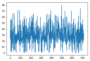
Since here only one data series was used, matplotlib uses these values as y-coordinates and the index of the sample as x-coordinate. Instead of plotting the data samples as a graph, we can use hist() to compute and show a histogram of the ages. In the next cell also labels are added to the plot.

plt.hist(ages)
plt.xlabel('age')
plt.ylabel('count')
plt.show()

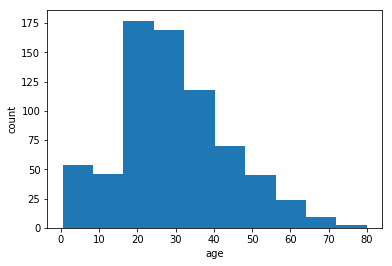
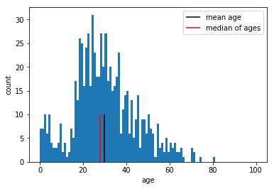
In the next cell, we further improve the plot by specifying the histogram range and the bin size. Additionally mean and median age are drawn and labeled.

plt.hist(ages, bins=100, range = [0,100])
plt.vlines([mean_age], 0 , 10, label='mean age', color='black')
plt.vlines([median], 0 , 10, label='median of ages', color='red')
plt.legend()
plt.xlabel('age')
plt.ylabel('count')
plt.show()

Sometimes we want to have a different plot size inside the notebooks. this can be achieved using the following code.

from matplotlib import rcParams
rcParams['figure.figsize'] = [10, 10] # with and height of plots (default is 6,4 )

For further information on matplotlib you may continue here.

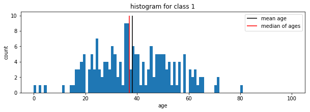
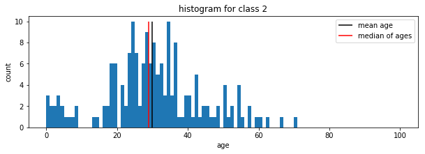
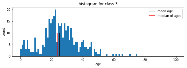
Exercise

Plot the age histogram for passengers with class 1,2 and 3 individually. You can create a subset of ages corresponding to a certain class using ages_i = np_ages[np_pclasses==i] where i denotes the class as integer or float number.

'''
np_pclasses = np.array(pclasses)
'''
### BEGIN SOLUTION
np_pclasses = np.array(pclasses)
for i in [1,2,3]:
    plt.subplot(3,1,i)
    plt.title(f'histogram for class {i}')
    ages_i = np_ages[np_pclasses==i]
    mean_age_i = np.mean(ages_i)
    median_i = np.median(ages_i)
    plt.hist( np_ages[np_pclasses==i], bins=100, range = [0,100])
    plt.vlines([mean_age_i], 0 , 10, label='mean age', color='black')
    plt.vlines([median_i], 0 , 10, label='median of ages', color='red')
    plt.legend()
    plt.xlabel('age')
    plt.ylabel('count')
    plt.show()
### END SOLUTION

Saving figures

Saving figures is quite easy as shown in the next cell. It only requires to replace plt.show() with plt.savefig() where the argument fname denotes the output file name.

rcParams['figure.figsize'] = [6, 4] # with and height of plots (default is 6,4 )

plt.hist(ages, bins=100, range = [0,100])
plt.vlines([mean_age], 0 , 10, label='mean age', color='black')
plt.vlines([median], 0 , 10, label='median of ages', color='red')
plt.legend()
plt.xlabel('age')
plt.ylabel('count')
plt.savefig(fname='figure')

Following cell removes the input/output promts to the left of the cells. Output scroll toggle via ctrl-o.

%%HTML
<style>div.prompt {display:none}</style>