Linear Regression
Using Python and Scipy
This page can be downloaded as interactive jupyter notebook
In this notebook, we use the scipy module to perform a linear regression in Python. Assuming we have a set of 2D points $(x,y)$ we want to regress the parameters $a, b$ of the linear equation $y = a\cdot x + b$ such that the mean squared error of $y$ w.r.t. all samples is minimal.
Preparation
In order to implement the regression, we first import the required Python modules:
import numpy as np                          # Used for numerical computations
from scipy.stats import linregress          # Implementation of the regression
import matplotlib.pyplot as plt             # Plotting library

# This is to set the size of the plots in the notebook
plt.rcParams['figure.figsize'] = [6, 6]
Creating a Toy Dataset
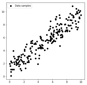
Next, we will create a toy dataset. It will contain noisy samples drawn from a known line.
ar, br = 0.873, 1.243                          # Ground truth parameters

np.random.seed(0)
x = np.random.random(200)*10                 # Drawing 500 points in the range [0,10]
y = ar*x + br + np.random.randn(200)           # We compute the y coordinates with a additional white noise

plt.scatter(x, y, c='black', marker='o', label='Data samples')
plt.legend(); plt.show()
Performing the regression
The linear regression using scipy can be done in one line. The function will return:
a: slopeb: interceptr: correlation coefficientp: p-value for a hypothesis tests: standard error of the estimated gradient
a,b,r,p,s = linregress(x,y)
print('slope:', a)
print('intercept:', b)
print('correlation coefficient:', r)
print('p-value:', p)
print('standard error of the estimated gradient:', s)
slope: 0.8291955978325258
intercept: 1.3499418955427611
correlation coefficient: 0.9265832004752252
p-value: 4.938058020631706e-86
standard error of the estimated gradient: 0.023918369974605936
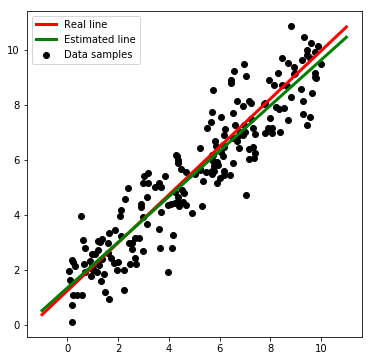
We can see that the correlation coefficient is close to 1.0 which means that the correlation is very high and it is thus very likely, that a linear relation exists. For visualization we can draw the real and estimated lines:
ar, br = 0.873, 1.243                          # Ground truth parameters

plt.scatter(x, y, c='black', marker='o', label='Data samples')

x_line = np.array([-1.0, 11.0])
real_y = ar*x_line + br
esti_y = a*x_line + b

plt.plot(x_line, real_y,c='red',lw=3, label='Real line')
plt.plot(x_line, esti_y,c='green',lw=3, label='Estimated line')

plt.legend(); plt.show()
| Author: | Dennis Wittich |
| Last modified: | 06.05.2019 |