Non-parametric classification:

Using Kernel Density Estimation and K Nearest Neighbours

This page can be downloaded as interactive jupyter notebook

In this notebook, we implement two non-parametric classification approaches: Kernel Density Estimation (KDE) and K Nearest Neighbours (KNN). Both approaches are based on the assumption that the probability of a sample $x$ for belonging to class $k$ can be approximated as

$p(x \mid C=L^k)\approx \dfrac{K_k}{N_k \cdot V}$

where

$V$ is a volume around $x$
$N_k$ is the number of training samples of class $k$
$K_k$ is the number of training samples of class $k$ that fall into $V$

In order to evaluate $K_k$, all training samples have to be accessible, which is a drawback of these approaches.

Preparation

In order to implement the algorithm, we first import the required Python modules:

import numpy as np                          # Used for numerical computations
import matplotlib.pyplot as plt             # Plotting library  

# This is to set the size of the plots in the notebook
plt.rcParams['figure.figsize'] = [6, 6]

Creating a Toy Dataset

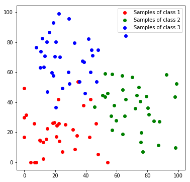
Next, we will create a toy dataset. It will contain samples which are drawn from 3 normal distributions, where each distribution represents a class.

num_c = 3 # Number of clusters
colours = [[255, 170, 170], [170, 255, 170], [170, 170, 255]]

# Generate the samples (3 clusters), we set a fixed seed make the results reproducable
np.random.seed(0)
c1_samples = np.clip([(20, 20) + np.random.randn(2)*15 for i in range(33)], 0, 100)
c2_samples = np.clip([(70, 30) + np.random.randn(2)*15 for i in range(33)], 0, 100)
c3_samples = np.clip([(30, 70) + np.random.randn(2)*15 for i in range(33)], 0, 100)

# Plot the samples, colored by class
plt.scatter(*zip(*c1_samples), c='red', marker='o', label='Samples of class 1')
plt.scatter(*zip(*c2_samples), c='green', marker='o', label='Samples of class 2')
plt.scatter(*zip(*c3_samples), c='blue', marker='o', label='Samples of class 3')
plt.legend()
plt.show()

png

We stack all data samples to one matrix and append the class index as additional column. Each row in the resulting matrix contains one the x and y coordinates and the class index of one sample.

c1_array = np.hstack((np.array(c1_samples), 1 * np.ones((len(c1_samples), 1))))
c2_array = np.hstack((np.array(c2_samples), 2 * np.ones((len(c2_samples), 1))))
c3_array = np.hstack((np.array(c3_samples), 3 * np.ones((len(c3_samples), 1))))

all_samples = np.vstack((c1_array, c2_array, c3_array))
print('Shape of stacked sample matrix:', all_samples.shape)

Shape of stacked sample matrix: (99, 3)

KDE-Classification

In Kernel Density Estimation, the idea is to fix the control volume $V$ and count the number of samples per class, that fall into the volume. Usually the counting is done in a smoothed way via a kernel function. This function acts as a measurement of contribution of each sample to the region of interest. The closer a sample $x_i$ is to the feature $x$ which is to be classified, the higher the contribution. Here we use a multivariate normal distribution

$k(x_i\mid x,\sigma^2 ) = \dfrac{1}{\sqrt{(2\pi)^n det(\Sigma)}}\cdot exp(-\dfrac{1}{2}(x_i-x)^T\Sigma^{-1}(x_i-x))$

where $\sigma$ defines the band with and thus corresponds to the size of $V$ and $n$ is the number of features (here 2).

def gaussian_kernel(x, x_i, sigma):
    Sigma = np.eye(2)*sigma # we do not consider covariances here
    inv = np.linalg.inv(Sigma)
    det = np.linalg.det(Sigma)
    dif = x_i-x[:,:2]
    return 1 / (np.sqrt((2*np.pi)**len(x)*det)) * np.exp(-0.5* np.sum((dif@inv)*(dif), axis=1))

In order to predict the class of a new feature $x$ we compute the conditional probability

$p(x\mid C=L^k) = \dfrac{1}{N_k}\cdot \sum\limits_{i=1}^{N_k}k(x_i

x,\sigma^2 )$

for all classes and return the most probable class.

def predict_kde(x, data, sigma):
    weights = gaussian_kernel(data, x, sigma)
    classes = list(set(data[:,2]))
    sums = [np.sum(weights[data[:,2]==c]) for c in classes]
    counts = [np.sum(data[:,2]==c) for c in classes]
    return np.argmax(np.array(sums)/np.array(counts))

Evaluation

To visualize the decision boundaries we predict every feature of the feature space.

def predict_feature_space_kde(data, sigma):
    label_map = np.zeros((100, 100, 3), dtype=np.ubyte)
    for x in range(100):
        for y in range(100):
            label = predict_kde(np.array((x, y), dtype=np.float), data, sigma)
            label_map[y, x] = colours[label]
    return label_map

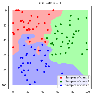
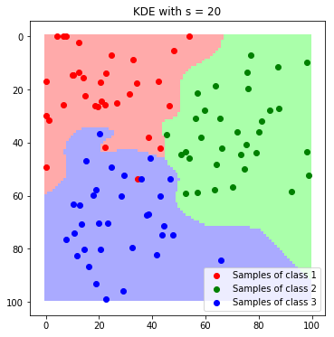
We evaluate the algorithm for different values for $\sigma$.

label_map_sigma_1 = predict_feature_space_kde(all_samples, 1)
label_map_sigma_20 = predict_feature_space_kde(all_samples, 20)
label_map_sigma_50 = predict_feature_space_kde(all_samples, 50)

plt.imshow(label_map_sigma_1)
plt.scatter(*zip(*c1_samples), c='red', marker='o', label='Samples of class 1')
plt.scatter(*zip(*c2_samples), c='green', marker='o', label='Samples of class 2')
plt.scatter(*zip(*c3_samples), c='blue', marker='o', label='Samples of class 3')
plt.title('KDE with s = 1'); plt.legend(); plt.show()

png

plt.imshow(label_map_sigma_20)
plt.scatter(*zip(*c1_samples), c='red', marker='o', label='Samples of class 1')
plt.scatter(*zip(*c2_samples), c='green', marker='o', label='Samples of class 2')
plt.scatter(*zip(*c3_samples), c='blue', marker='o', label='Samples of class 3')
plt.title('KDE with s = 20'); plt.legend(); plt.show()

png

plt.imshow(label_map_sigma_50)
plt.scatter(*zip(*c1_samples), c='red', marker='o', label='Samples of class 1')
plt.scatter(*zip(*c2_samples), c='green', marker='o', label='Samples of class 2')
plt.scatter(*zip(*c3_samples), c='blue', marker='o', label='Samples of class 3')
plt.title('KDE with s = 50'); plt.legend(); plt.show()

png

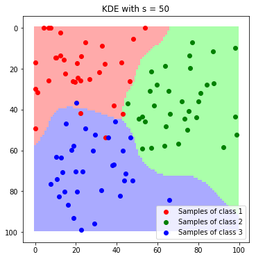
We can nicely see how the resulting boundaries get smoother as we increase the band with $\sigma$.

KNN-Classification

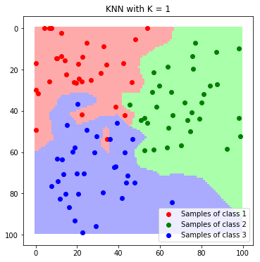
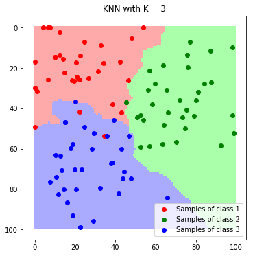
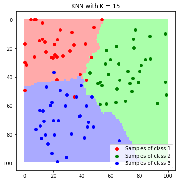
The idea behind the K Nearest Neighbour classification is to freeze the number of neighbours per class and measure the minimum size of the required control volume that is required to include all of them. However, here we use the direct classification, where we simply take the K nearest neighbours and assign the most frequent class among these samples.

def predict_knn(x, data, K):
    num_samples = data.shape[0]
    distances = np.array([np.sqrt(np.sum((x-data[i, :2])**2)) for i in range(num_samples)])
    K_nearest_neighbours = np.argsort(distances)[:K]
    nearest_classes = data[K_nearest_neighbours, 2].astype(np.int)
    return np.argmax(np.bincount(nearest_classes))

Evaluation

Again, we classify each feature in the feature space to visualize the decision boundaries..

def predict_feature_space_knn(data, K):
    label_map = np.zeros((100, 100, 3), dtype=np.ubyte)
    for x in range(100):
        for y in range(100):
            label = predict_knn(np.array((x, y), dtype=np.float), data, K)
            label_map[y, x] = colours[label-1]
    return label_map

.. and evaluate the method. This time with different values for the number of neighbours $K$.

label_map_K1 = predict_feature_space_knn(all_samples, 1)
label_map_K3 = predict_feature_space_knn(all_samples, 3)
label_map_K15 = predict_feature_space_knn(all_samples, 15)

plt.imshow(label_map_K1)
plt.scatter(*zip(*c1_samples), c='red', marker='o', label='Samples of class 1')
plt.scatter(*zip(*c2_samples), c='green', marker='o', label='Samples of class 2')
plt.scatter(*zip(*c3_samples), c='blue', marker='o', label='Samples of class 3')
plt.title('KNN with K = 1'); plt.legend(); plt.show()

png

plt.imshow(label_map_K3)
plt.scatter(*zip(*c1_samples), c='red', marker='o', label='Samples of class 1')
plt.scatter(*zip(*c2_samples), c='green', marker='o', label='Samples of class 2')
plt.scatter(*zip(*c3_samples), c='blue', marker='o', label='Samples of class 3')
plt.title('KNN with K = 3'); plt.legend(); plt.show()

png

plt.imshow(label_map_K15)
plt.scatter(*zip(*c1_samples), c='red', marker='o', label='Samples of class 1')
plt.scatter(*zip(*c2_samples), c='green', marker='o', label='Samples of class 2')
plt.scatter(*zip(*c3_samples), c='blue', marker='o', label='Samples of class 3')
plt.title('KNN with K = 15'); plt.legend(); plt.show()

png

Discussion

In this example, both are suitable for classification if the hyper-parameters are set properly. Since each method only has one hyper-parameter they are easy tunable and they do not require any training. Again, a drawback is that all data has to be ready in memory and the implementation can have a major impact on the runtime!

Author:	Dennis Wittich
Last modified:	06.05.2019